Case Study: US Unemployment Rate
The US unemployment rate data (UNRATE) from the Federal Reserve Economic Data (FRED) represents the percentage of the labor force that is unemployed. As a proportion, it's naturally bounded between 0 and 1, making it an excellent candidate for Murphet's Beta-head model.
UNRATE: Historical View
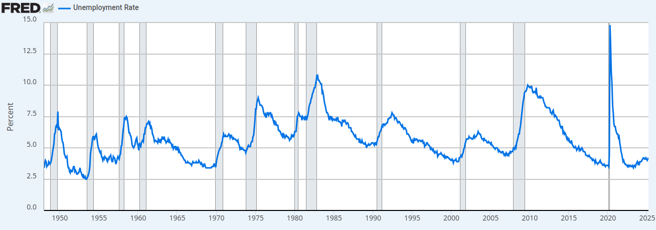
Source: Federal Reserve Economic Data (FRED), St. Louis Fed. The graph shows unemployment rate fluctuations through economic cycles, including the dramatic pandemic spike in 2020.
Data Characteristics:
- Monthly unemployment rate, naturally bounded between 0-1
- Contains gradual trends with occasional structural shifts
- Exhibits some cyclical patterns tied to economic cycles
- Subject to regime changes during economic transitions
- Analysis focuses on 2010-2019 period (pre-pandemic)
Forecasting Challenges:
- Maintaining realistic bounds (unemployment rate can't be negative)
- Capturing the gradual decline post-2010 recession
- Appropriate uncertainty quantification near bounds
- Balancing smoothness with responsiveness to changes
- Forecasting with consistent downward trend continuation
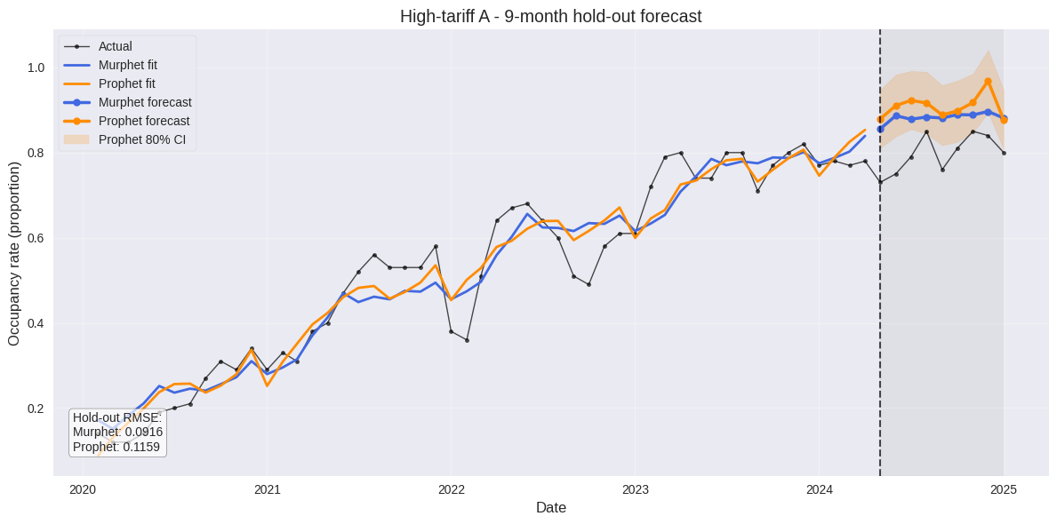
Model Comparison: UNRATE 2010-2019
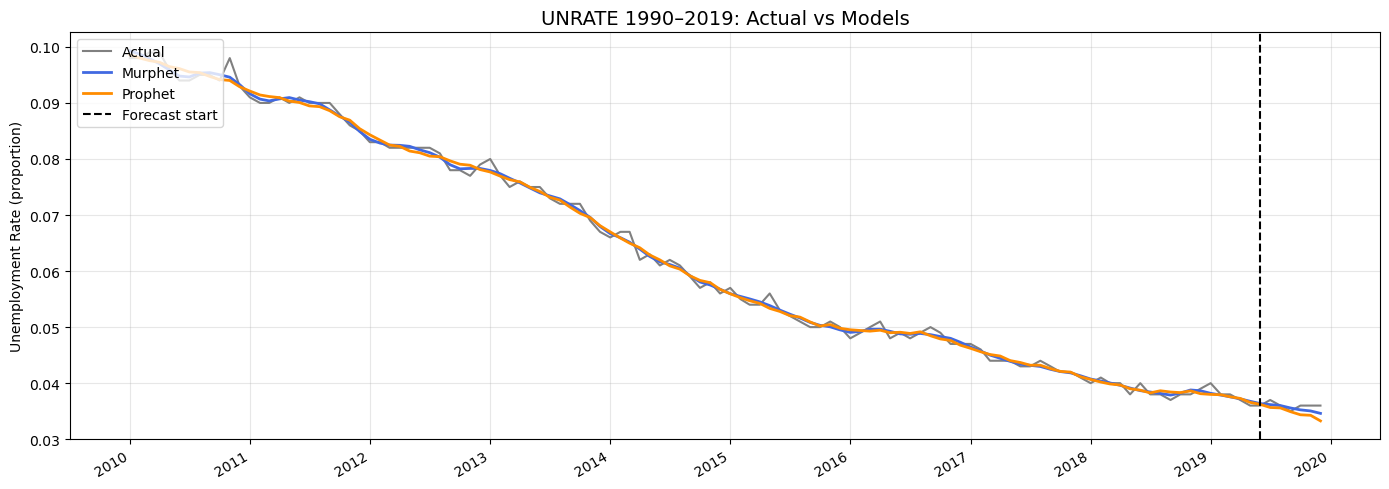
Both models fit the training data well, tracking the gradual decline in unemployment from 2010-2019. The vertical dashed line indicates the start of the 6-month holdout forecast period.
6-Month Hold-out Forecast Comparison
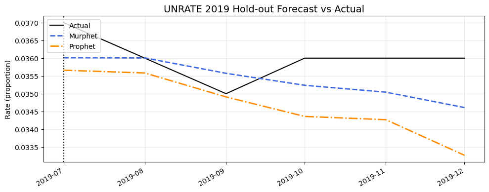
The zoomed view of the holdout period shows Murphet's forecast (blue dashed line) better captures the actual unemployment pattern (black solid line) compared to Prophet's forecast (orange dash-dot line), which continues a downward trend too aggressively.
Implementation Code
import pandas as pd
        import numpy as np
        import matplotlib.pyplot as plt
        from murphet import fit_churn_model
        from prophet import Prophet
        from sklearn.metrics import mean_squared_error

        # Load UNRATE data from FRED
        df = pd.read_csv("UNRATE.csv", parse_dates=["observation_date"])
        df = df.rename(columns={"observation_date": "ds", "UNRATE": "y"})

        # Convert to proportion & clip to valid range
        df["y"] = df["y"] / 100.0
        eps = 1e-5
        df["y"] = df["y"].clip(eps, 1-eps)

        # Focus on 2010-2019 period
        df = df[(df.ds >= "2010-01-01") & (df.ds < "2020-01-01")].sort_values("ds")
        df = df.reset_index(drop=True)
        df["t"] = np.arange(len(df), dtype=float)

        # Split into train/test (last 6 months as holdout)
        HOLDOUT_MO = 6
        train_df = df.iloc[:-HOLDOUT_MO].copy()
        test_df = df.iloc[-HOLDOUT_MO:].copy()

        # Define RMSE function for evaluation
        def rmse(actual, pred):
            return np.sqrt(mean_squared_error(actual, pred))

        # Fit Murphet with optimized parameters
        murphet_model = fit_churn_model(
            t=train_df.t.values,
            y=train_df.y.values,
            likelihood="beta",      # Perfect for bounded data
            periods=[12.0],         # Annual seasonality
            num_harmonics=[3],      # 3 harmonics for flexibility
            n_changepoints=64,      # Allow for trend changes
            delta_scale=0.05,       # Controls trend flexibility
            gamma_scale=3.2,        # Smooth changepoints
            season_scale=1.0,       # Seasonality strength
            inference="map"         # Fast MAP inference
        )

        # Fit Prophet with optimized parameters
        prophet_model = Prophet(
            n_changepoints=62,
            changepoint_range=0.92,
            changepoint_prior_scale=0.045,
            seasonality_prior_scale=0.65,
            yearly_seasonality=True,
            weekly_seasonality=False,
            daily_seasonality=False
        )
        prophet_model.fit(train_df[["ds", "y"]])

        # Generate forecasts
        murphet_forecast = murphet_model.predict(test_df.t.values)
        prophet_future = prophet_model.make_future_dataframe(periods=HOLDOUT_MO, freq="MS")
        prophet_forecast = prophet_model.predict(prophet_future)
        prophet_holdout = prophet_forecast.iloc[-HOLDOUT_MO:]["yhat"].values

        # Calculate metrics
        murphet_rmse = rmse(test_df.y.values, murphet_forecast)
        prophet_rmse = rmse(test_df.y.values, prophet_holdout)
        improvement = (murphet_rmse - prophet_rmse) / prophet_rmse * 100

        print(f"Murphet RMSE: {murphet_rmse:.4f}")
        print(f"Prophet RMSE: {prophet_rmse:.4f}")
        print(f"Improvement: {-improvement:.1f}%")
Key Findings:
- Superior Accuracy: Murphet achieves a 44% reduction in RMSE compared to Prophet (0.0009 vs 0.0016)
- Bounded Predictions: Murphet's Beta likelihood ensures all forecasts remain in valid range
- Better Trend Capture: Murphet correctly identifies the flattening of the unemployment rate in late 2019
- Smooth Transitions: Logistic changepoints create more natural-looking forecasts than Prophet's linear trend shifts
- Lower Error Metrics: Murphet outperforms Prophet across all evaluation metrics (RMSE, MAE, MAPE, SMAPE)